
Background:
Background
In High Temperature Superconductors (HTS), “quench” occurs when (for a variety of reasons) the superconducting material abruptly loses its superconductivity. This results in a huge increase in voltage across the material, and if the current isn’t shut off immediately the resistive heat generated can destroy the superconductor. Quench detection is one of the most pertinent research fields related to making HTS more accessible and widespread. Current quench detection methods involve using voltage sensors and electromagnetic field detectors. However there are considerable drawbacks to these methods, including slow response time, sensitivity, and cost.
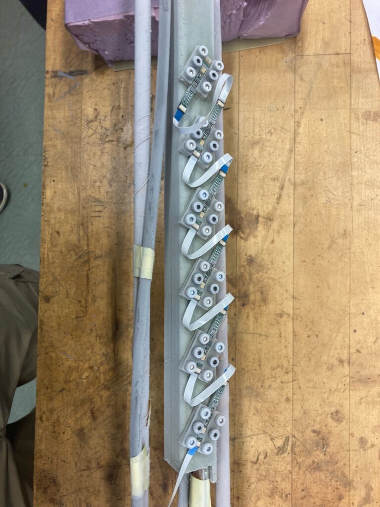
My research advisor proposes a method of detecting superconductor quench event using Microelectromechanical Systems (MEMS) microphones placed in the cryogenic chamber with the superconducting material. These microphones would be able to pick up acoustic pressure waves given off by the early stages of a quench event faster than current quench detection methods. Since these microphones are designed and fabricated in the lab, significant testing must be done to validate them.
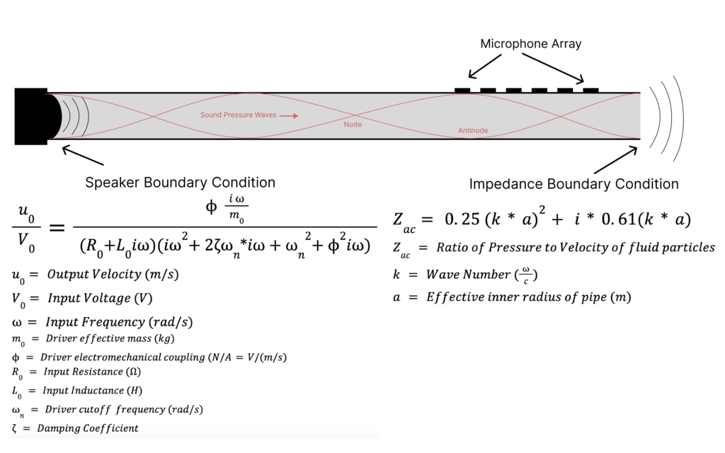
One of the validation methods my research advisor proposed was inserting a small speaker into one end of the tube which houses the microphone and sweeping through a series of frequencies of sine waves to see if the microphones can read the standing waves in the tube. In order to have reference values for this test we must be able to predict the pressure values at every point in the tube for each input frequency.
My Role:
My job was to develop an acoustic model of sound wave propagation in the tube in order to predict what pressures the MEMS microphones should be reading given an input frequency. Acoustic models are common and well documented, however this one was uniquely challenging for a few reasons:
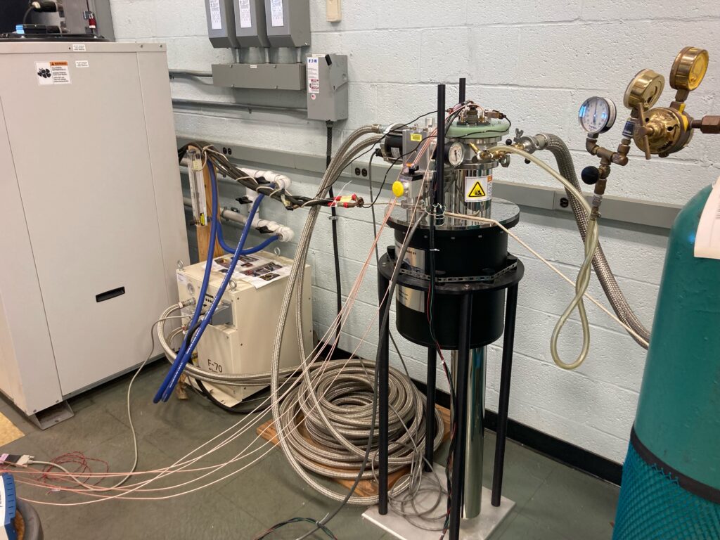
- There will be an extreme temperature gradient from one end of the tube to another, ranging from room temperature to as low as 50 degrees Kelvin. This means the speed of sound will be changing significantly along the length of the tube.
- An accurate damping model of cryogenic Helium needed to be incorporated.
- A transfer function of the speaker needed to be incorporated giving an output velocity for a given frequency and input voltage.
My Process
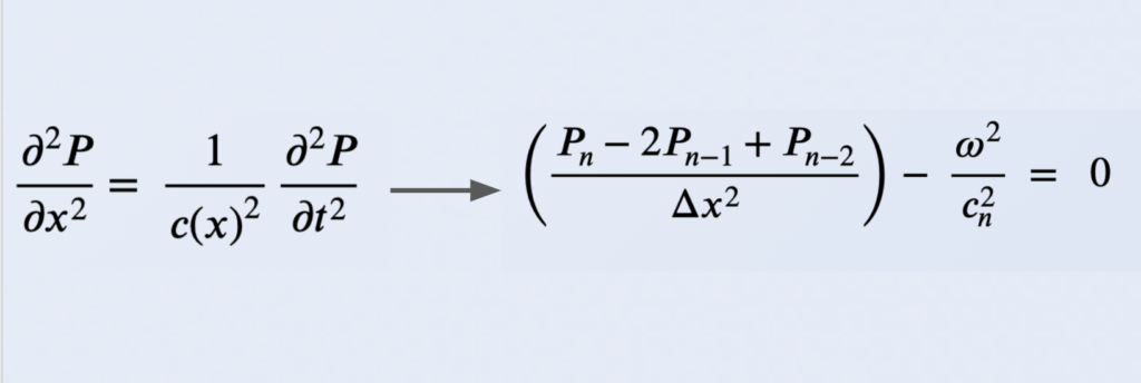
I used the finite difference method to solve the 1D wave equation by splitting the tube into infinitesimally small segments and solving for pressure at each point using matrix inversion. The 1D wave equation is shown below, with c(x) representing the speed of sound which changes as you move along the tube.
The time component of the equation can be removed by assuming a time harmonic solution (varies sinusoidally at input frequency). The left side of the equation is then replaced with the finite difference approximation of the double derivative of P with respect to x, leaving the following equation to be solved at each value of n:
An n by n matrix can then be constructed to solve for P at each point n. The first and last row of the matrix is defined by the boundary conditions and the rest of the rows are defined by above equation. Shown below is the setup of the matrix excluding the boundary conditions:
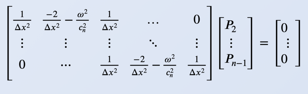
The boundary condition equations output velocity values, so the linearized Euler equation is used to convert velocity to pressure values. Once the pressure values for the boundary conditions have been solved they are inserted into the first and last rows of the matrices.
Damping:
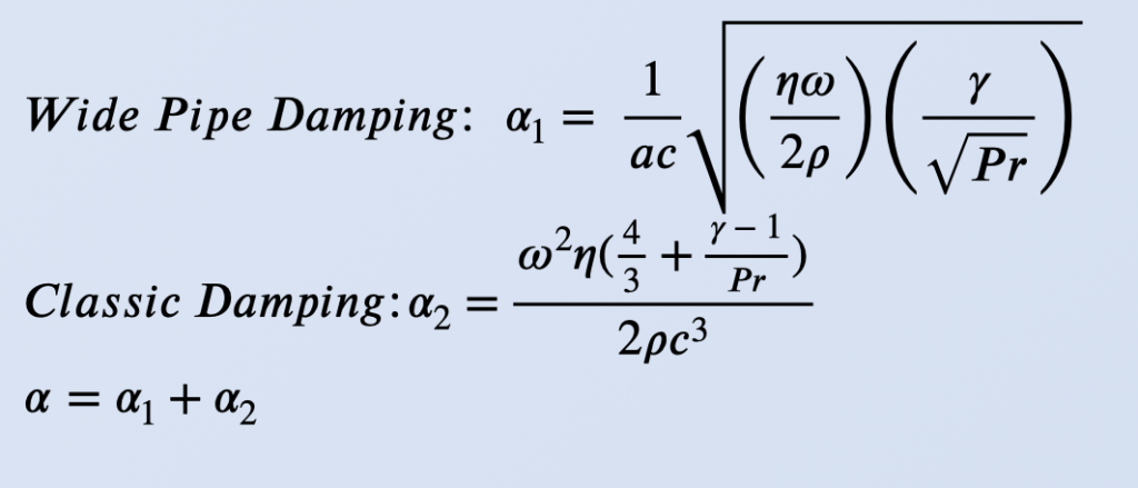
In order to accurately model propagation of pressure waves in the tube, a combination of classic and wide pipe damping was incorporated by multiplying the damping value alpha into the wave number k.
Temperature Gradient:
The temperature gradient in the tube was approximated by using an Akima cubic function to interpolate experimental measurements of temperature along the tube with a given end temperatures.
Results
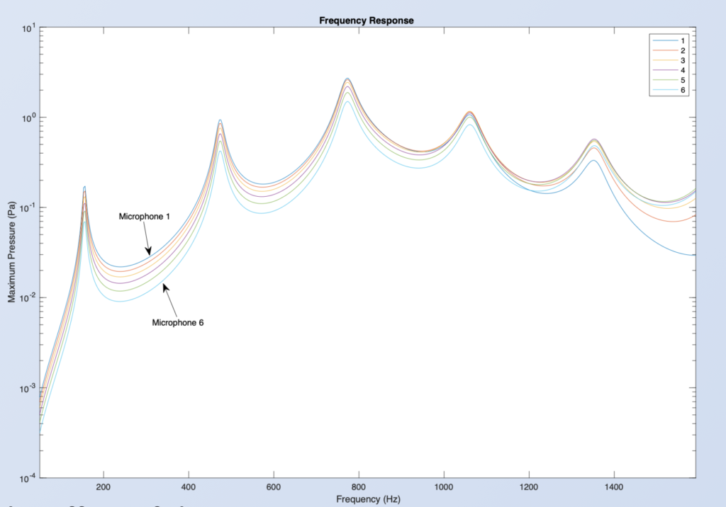
The resulting output of the model gives maximum pressure readings for each microphone at a wide range of input frequencies. In this example, the temperature at the end of the tube is 100K.
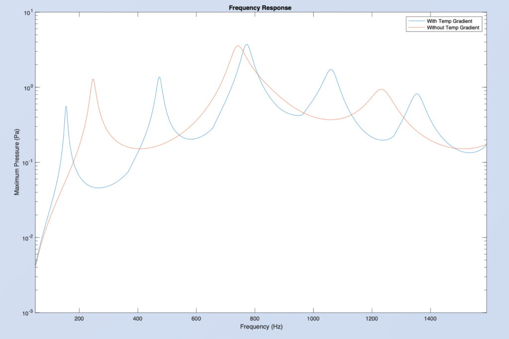
The effect of the temperature gradient on frequency response can be observed by comparing the results with and without the temperature gradient:
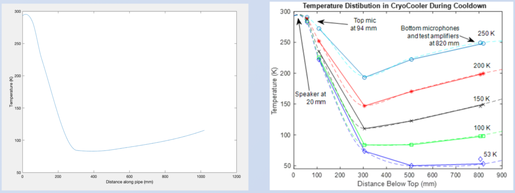
The interpolated temperature gradient with the end of the tube at 100K is compared to experimental data of temperature gradients in the cryocooler:
Code: (Matlab)
%u0 = 0.001; %m/s
w = linspace(1,10000,500); %rad/s
res = 1000;
x = linspace(0,1.02,res);
dx = x(2)-x(1);
endTemp = 100; %Kelvin
mics = [0.8395,0.861,0.8825,0.904,0.9255,0.947];% Microphone Positions (m)
T=TempVsX((x)*1000,endTemp); %Modified Akima cubic interpolant using experimental data
%T = linspace(295,endTemp,res); %Linear Temperature Gradient
zAir = 20.04; %Constant for speed of sound gradient (m/sK^1/2)
              % from 343m/s at 20 deg
zHelium = 58.8;
c = zHelium*sqrt(T); %Speed of sound (m/s)
a = 0.0216/sqrt(pi); %Effective Inner radius of pipe for impedence

%HELIUM:
eta=5.01e-7*(T.^0.646); %Fit to data from Cryogenic Data Handbook
Pr=0.6; %Helium, not sensitive to temperature
gamma=5/3; %Helium at 300K (ideal monatomic gas)
p0 = 1; %Pressure in atm

%Will be a function of x:
rho=0.1664 *(p0)*(T/293.15); %density of helium (kg/m^3)

%Driver Variables
V0=0.02; %Drive voltage to speaker (Vp)
Phi=2.1; %Driver electromechanical coupling (N/A=V/(m/s))
m0=1e-3; %Driver effective mass (kg)
R0=6.8; %Input resistance (Ohm)
L0=3.7e-5; %Input inductance (H)
wn=820*2*pi; %Driver cut-on frequency (Hz) HELIUM
%wn1=740*2*pi; %Drive cut-on frequench (Hz) AIR
zeta=0.085; %Driver damping HELIUM
%zeta1=0.09; %Drive damping AIR

%Driver model
u0=V0*(Phi.*1j*w./m0)./((R0+L0.*1j*w).*((1j*w).^2+2*zeta*wn.*1j*w+wn.^2)+(Phi^2).*(1j*w./m0));

%Initialize vectors which will hold max pressure values for each frequency
bodegradient = zeros(1,length(w));
bodeNogradient = zeros(1,length(w));
mic_mags = zeros(6,length(w));

%Sweep through the input frequencies
for i=1:length(w)


    % Speaker Boundary Condition:
    dPdx = -rho(1)*1j*w(i)*u0(i);

    %Damping:
    %will be a function of x:
    alpha_pipe=(1./(a*c)).*sqrt(eta.*w(i)./(2*rho))*(1+(gamma-1)/sqrt(Pr)); %wide pipe, Kinsler p. 233, alpha for wide pipe
    alpha_classic=w(i)^2.*eta.*(4/3+(gamma-1)/Pr)/(2.*rho.*c.^3); %Kinsler p. 218
    alpha=alpha_pipe+alpha_classic;


    P = zeros(res,1); %Pressure Values
    B = zeros(res,1); %Boundary  Conditions
    M = zeros(res, res); %Finite Difference Matrix

    % First row of the matrix, with speaker boundary condition moved to the right
    % side of the matrix equation
    k = w(i)/c(1) - 1j*alpha(1); %Wave number, including damping
%     M(1,1) = -2/(dx^2) + k^2;
%     M(1,2) = 1/(dx^2);

    M(1,1) = -1/(2*(dx^2));
    M(1,2) = 1/(2*(dx^2));

    % Rest of the matrix, defined by using Finite difference method to take
    % second derivative of pressure with respect to x
        for j=2:length(x)-1
             k = w(i)/c(j) - 1j*alpha(i);
             M(j,j-1) = 1/(dx^2);
             M(j,j) = -2/(dx^2) + k^2;
             M(j,j+1) = 1/(dx^2);
        end

    %Last row of the Matrix, with impedence boundary condition moved to the
    %right side of the matrix equation

    % Impedence Boundary condition
    Zac=(0.25*(k*a)^2+1j*0.61*k*a);

    %k = w(i)/c(res) - 1j*alpha(res);
%     M(res,res) = -2/(dx^2) + k^2;
%     M(res,res-1) = 1/(dx^2);
    M(res,res-1) = -Zac/(rho(res-1)*j*w(i)*dx);
    M(res,res) = 1 + Zac/(rho(res-1)*j*w(i)*dx);


    %Boundary conditions at both ends of the pipe
%     B(1) = -u0/(dx^2);
     %B(res) = -Zac/(dx^2);

    B(1) = dPdx/(2*dx);
    B(res) = 0;

    %Magnitude of the complex number of the pressure values
    P = abs(M\B);

    for n = 1:6
       [minValue,index] = min(abs(x-mics(n)));
        mic_mags(n,i) = P(index);
    end


    bodegradient(i) = max(P);


    %% NO Temp Gradient


    cHelium=1007;
    %cHelium = 343;
    M = zeros(res, res);

    k = w(i)/cHelium - 1j*alpha(1);
%     M(1,1) = -2/(dx^2) + k^2;
%     M(1,2) = 1/(dx^2);
    M(1,1) = -1/(2*(dx^2));
    M(1,2) = 1/(2*(dx^2));

    for j=2:length(x)-1
        k = w(i)/cHelium - 1j*alpha(i);
        M(j,j-1) = 1/(dx^2);
        M(j,j) = -2/(dx^2) + k^2;
        M(j,j+1) = 1/(dx^2);
    end

%     k = w(i)/cAir - 1j*alpha(res);
%     M(res,res) = -2/(dx^2) + k^2;
%     M(res,res-1) = 1/(dx^2);

    M(res,res-1) = -Zac/(rho(res-1)*j*w(i)*dx);
    M(res,res) = 1 + Zac/(rho(res-1)*j*w(i)*dx);

    Pideal = abs(M\B);
    bodeNogradient(i) = max(Pideal);

end

%semilogy(w/2/pi,bodegradient)
semilogy(w/2/pi,mic_mags(1,:))
hold on
semilogy(w/2/pi,mic_mags(2,:))
semilogy(w/2/pi,mic_mags(3,:))
semilogy(w/2/pi,mic_mags(4,:))
semilogy(w/2/pi,mic_mags(5,:))
semilogy(w/2/pi,mic_mags(6,:))
%semilogy(w/2/pi,bodeNogradient)
legend("With Temp Gradient","Without Temp Gradient")
%legend("1","2","3","4","5","6")
title("Frequency Response ")
xlabel("Frequency (Hz)")
ylabel("Maximum Pressure (Pa)")
xlim([50, w(end)/2/pi])
hold off

figure
plot(x*1000,T)
xlabel("Distance along pipe (mm)")
ylabel("Temperature (K)")

function T=TempVsX(x_mm,T820)


V=[ 293 293 293 293 293 293;...
    293 291 272.2790 193.0010  222.2450  248.1820;...
    293 288.5 251.8680 146.9230  170.3790  199.4750;...
    293 287.5 235.3040 109.9900  122.6490  149.2160;...
    293 284.2 225.4390 83.6007   83.9762   98.0037;...
    293 283 222.1850 73.6862   50.1674   53.1959];

[X,Y]=meshgrid([0 55 107.9500  304.8000  508.0000  818.6420],[293;248.2;199.5;149.2;98.0;53.2]);

T=interp2(X,Y,V,x_mm,T820,'makima');
end